![[论文理解] Classifier-Free Diffusion Guidance](https://sunlin-ai.github.io/images/albumsbg.jpg)
Classifier-free diffusion guidance1 可以显著提高样本生成质量,实施起来也十分简单高效,它也是 OpenAI’s GLIDE2 , OpenAI’s DALL·E 23 和 Google’s Imagen4的核心部分, 在这篇博客里我将分享它是如何工作的,部分内容参考5。
研究背景
仅仅两年前,扩散模型 还未引起广泛关注,但今天,扩散模型是图像和音频生成的首选模型。在之前的博客里,探讨了 guided_diffusion6,如果你还不熟悉这部分内容,推荐首先阅读 这篇博客7。
扩散模型是生成模型的一种,其对高维数据的分布 \(p(x)\) 建模,不同于直接估计 \(p(x)\) (likelihood-based models 的做法), 扩散模型尝试估计 score function \(\nabla_x \log p(x)\)。
使用扩散模型生成样本时, 输入随机噪声, 然后逐步去除噪声,普遍使用的解噪方法是 Stochastic Gradient Langevin Dynamics (SGLD) 。
在条件扩散模型中, 会有一个额外的输入 \(y\) (比如类别标签或者一段文字),我们尝试对条件概率分布 \(p(x \mid y)\) 建模, 在实做上,我们会建立模型来预测 score function \(\nabla_x \log p(x \mid y)\) ,这样做的好处是 score function 不依赖分布的标准化常数,因为 \(p(x) = \frac{\tilde{p}(x)}{Z}\),如果我们仅知道非规范化的概率分布 \(\tilde{p}(x)\),依然可以计算其 score function:
\[\nabla_x \log \tilde{p}(x) = \nabla_x \log \left( p(x) \cdot Z \right) = \nabla_x \left( \log p(x) + \log Z \right) = \nabla_x \log p(x),\]上式中 \(Z = \int \tilde{p}(x) \mathrm{d} x\) 不依赖于 \(x\),其关于 \(x\) 的梯度为0。
在扩散模型中, \(\nabla_{\mathbf{x}} \log p\left(\mathbf{x}\right)=-\frac{1}{\sqrt{1-\bar{\alpha}}} \epsilon_{\theta}\left(\mathbf{x}\right)\) 6,所以通常将目标转化为求取 \(\epsilon_{\theta}\left(\mathbf{x}\right)\)。
理论推导
根据 DDIM 的采样过程:
\[\boldsymbol{x}_{t-1}=\sqrt{\alpha_{t-1}} \underbrace{\left(\frac{\boldsymbol{x}_{t}-\sqrt{1-\alpha_{t}} \epsilon_{\theta}^{(t)}\left(\boldsymbol{x}_{t}\mid \mathbf{y}\right)}{\sqrt{\alpha_{t}}}\right)}_{\text {"predicted } \boldsymbol{x}_{0} \text { " }}+\underbrace{\sqrt{1-\alpha_{t-1}} \cdot \epsilon_{\theta}^{(t)}\left(\boldsymbol{x}_{t}\mid \mathbf{y}\right)}_{\text {“direction pointing to } \boldsymbol{x}_{t} \text { " }},\]如果能得到 \(\epsilon_{\theta}\left(\mathbf{x_{t}} \mid \mathbf{y}\right)\) ,就可以使用上式生成图像,如何得到 \(\epsilon_{\theta}\left(\mathbf{x_{t}} \mid \mathbf{y}\right)\)?有2种方法:
Classifier guidance
根据贝叶斯公式:
\[p(\mathbf{x_{t}} \mid \mathbf{y}) = \frac{p(y \mid \mathbf{x_{t}}) \cdot p(\mathbf{x_{t}})}{p(\mathbf{y})}\] \[\implies \log p(\mathbf{x_t} \mid \mathbf{y}) = \log p(y \mid \mathbf{x_t}) + \log p(\mathbf{x_t}) - \log p(\mathbf{y})\]对上式两边同时求关于 \(\mathbf{x_t}\) 的导数,因为 \(\nabla_\mathbf{x_t} \log p(\mathbf{y}) = 0\), 所以:
\[\implies \nabla_\mathbf{x_t} \log p(\mathbf{x_t} \mid \mathbf{y}) = \nabla_\mathbf{x_t} \log p(\mathbf{x_{t}})+\nabla_\mathbf{x_t} \log p(\mathbf{y} \mid \mathbf{x_t})\]Dhariwal 和 Nichol6 发现 classifier guidance 可以通过增强条件信息,显著提高样本生成质量,为了实现这一点,在条件项上增加一个尺度因子:
\[\nabla_\mathbf{x_t} \log p(\mathbf{x_t} \mid \mathbf{y}) = \nabla_\mathbf{x_t} \log p(\mathbf{x_t}) + \gamma \nabla_\mathbf{x_t} \log p(\mathbf{y} \mid \mathbf{x_t}) .\]\(\gamma\) 称为 guidance scale, 当其取值大于1时,可以增大条件信息的影响,可以将概率质量从最不可能的值移动到最可能的值(即温度降低)来锐化分布,并聚焦到其模式上,这相比于 GANs8 的 truncation trick这个做法更加高效。
需要注意的是条件项 \(\nabla_\mathbf{x_{t}} \log p(\mathbf{y} \mid \mathbf{x_{t}})\)不是 score function, 因为它是关于 \(\mathbf{x_{t}}\) 的梯度而不是 \(\mathbf{y}\)。
因为 \(\nabla_{\mathbf{x}_t} \log p\left(\mathbf{x}_t\right)=-\frac{1}{\sqrt{1-\bar{\alpha}_t}} \epsilon\left(\mathbf{x}_t\right)\),所以:
\[-\frac{1}{\sqrt{1-\bar{\alpha}_t}} {\epsilon}_{\theta}\left(\mathbf{x_t\mid y}\right)=-\frac{1}{\sqrt{1-\bar{\alpha}_{t}}}\epsilon_{\theta}\left(\mathbf{x_t}\right)+\gamma\cdot\nabla_{\mathbf{x_t}} \log p_{\phi}\left(\mathbf{y} \mid \mathbf{x_t}\right),\] \[\implies \epsilon_{\theta}\left(\mathbf{x_t\mid y}\right):=\epsilon_{\theta}\left(\mathbf{x_t}\right)-\sqrt{1-\bar{\alpha}_t} \cdot\gamma\cdot\nabla_{\mathbf{x_t}} \log p_{\phi}\left(\mathbf{y} \mid \mathbf{x_t}\right).\]如果我们有一个可微分判别模型 \(p_{\phi}\left(\mathbf{y} \mid \mathbf{x_t}\right)\) 的,那我们就很容易得到 \(\nabla_{\mathbf{x_t}} \log p_{\phi}(\mathbf{y} \mid \mathbf{x_t})\)。 所以要将无条件扩散模型转换为条件扩散模型,我们所需要的只是一个分类器!
在语言模型中,通常预训练一个强大的无条件语言模型,在下游任务中,根据需要进行模型微调。从表面上看,classifier guidance 似乎为图像生成提供了同样的功能:预训练一个强大的无条件模型,然后在测试时使用单独的分类器,根据需要对分类器微调。
不幸的是,有一些障碍使这变得不切实际。最重要的是,由于扩散模型逐渐对输入噪声去噪,因此任何用于引导的分类器也需要能够应对高水平噪声,以便它可以在整个采样过程中提供有用的信息。这通常需要训练定制的分类器,在这一点上,端到端地训练传统条件生成模型更容易。
此外,即使我们有一个噪声鲁棒的分类器,classifier guidance 的有效性在本质上也是有限的:输入 \(\mathbf{x_t}\) 中的大多数信息与预测标签 \(\mathbf{y}\) 无关,因此,采用分类器关于其输入的梯度可以在输入空间中产生任意(甚至是对抗)的方向。
classifier-free guidance
\[\nabla_\mathbf{x_t} \log p(\mathbf{x_t} \mid \mathbf{y}) = \nabla_\mathbf{x_t} \log p(\mathbf{x_t})+ \nabla_\mathbf{x_t} \log p(\mathbf{x_t} \mid \mathbf{y}) - \nabla_\mathbf{x_t} \log p(\mathbf{x_t}) .\]为了在 classifier-free guidance 中使用通用文本prompts,在训练中有时会将文本替换为空序列(表示为 \(\emptyset\)),随后使用更新的 \(\epsilon_{\theta}\left(\mathbf{x_t} \mid \mathbf{y}\right)\) 指导生成标签为 \(\mathbf{y}\) 的图像:
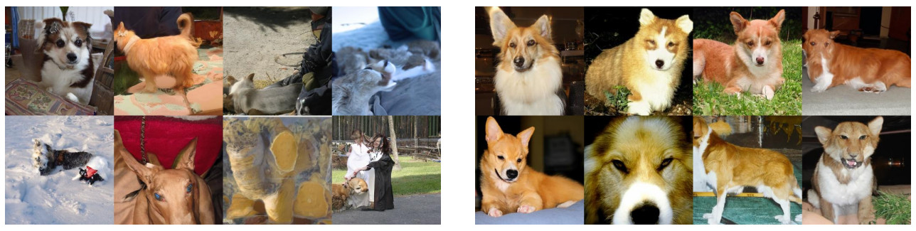
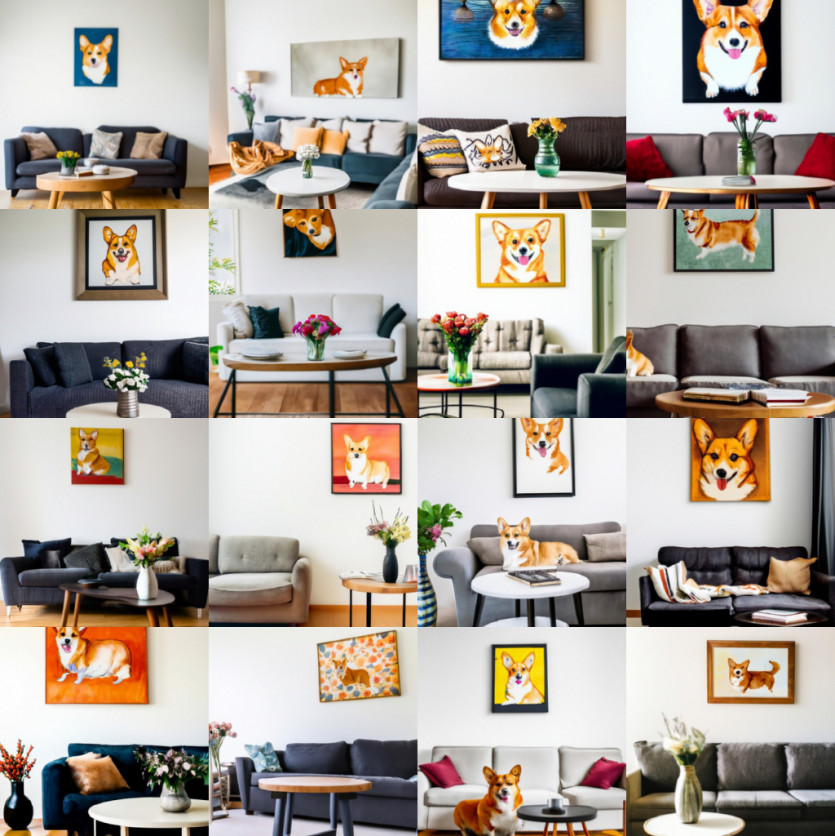
\[\implies\epsilon_{\theta}\left(\mathbf{x_t} \mid \mathbf{y}\right)=\epsilon_{\theta}\left(\mathbf{x_t} \mid \emptyset\right)+\gamma\cdot\left(\epsilon_{\theta}\left(\mathbf{x_t} \mid \mathbf{y}\right)-\epsilon_{\theta}\left(\mathbf{x_t} \mid \emptyset\right)\right),\]当 \(\gamma = 0\) 为无条件模型;当 \(\gamma = 1\) 为标准的条件概率模型。当 \(\gamma > 1\) 时,神奇的事情就发生了,以下是 OpenAI 的使用classifier-free guidance的 GLIDE model2例子:
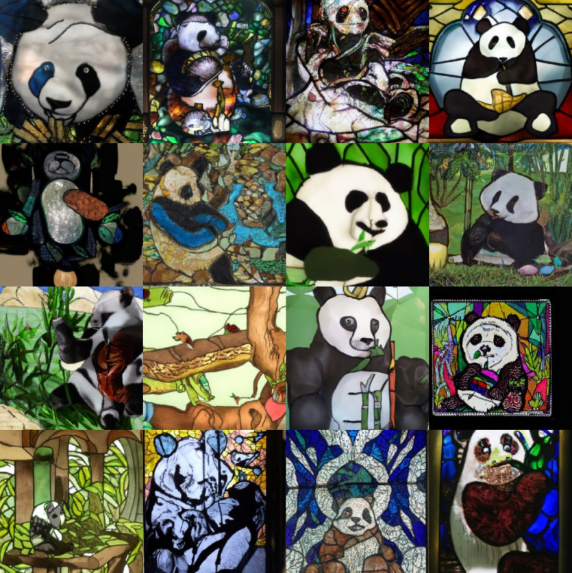
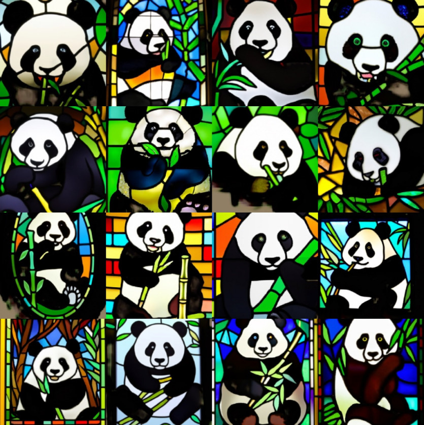
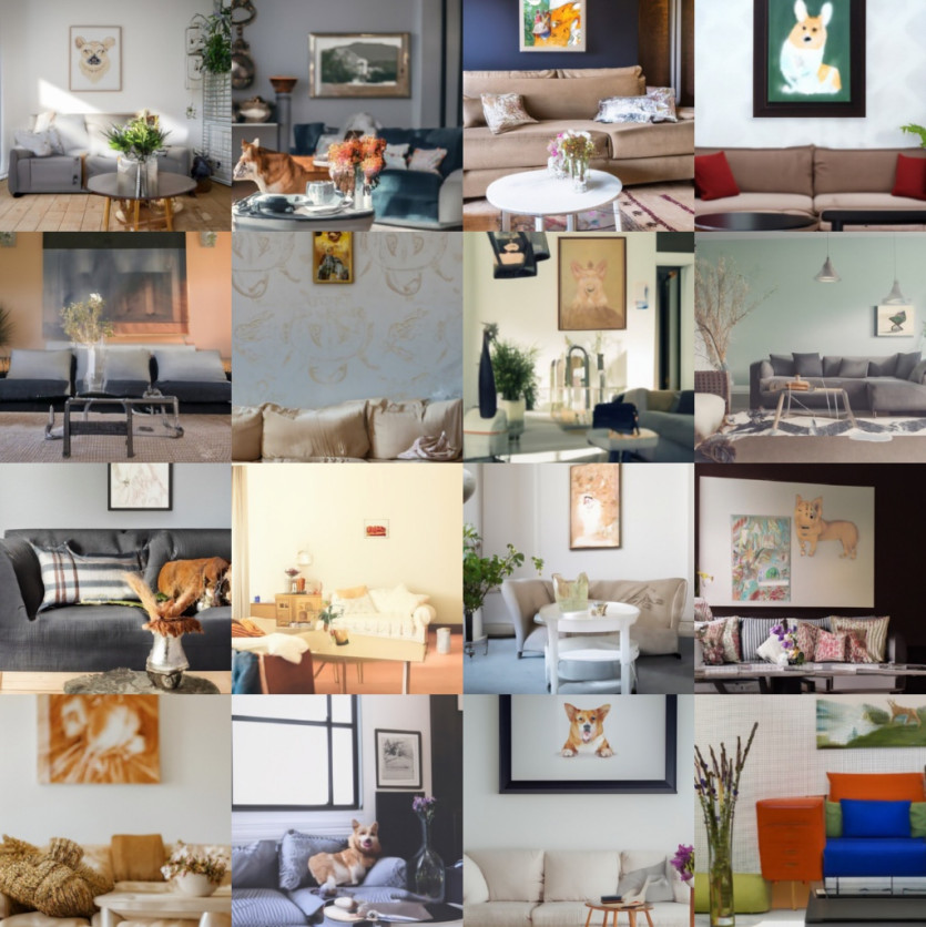
为什么这比 classifier guidance 好得多?主要原因是我们从生成模型构造了“分类器”,而标准分类器可以走捷径:忽视输入 \(x\) 依然可以获得有竞争力的分类结果,而生成模型不容易被糊弄,这使得得到的梯度更加稳健。
值得注意的是,classifier-free guidance的想法发布和 OpenAI 的 GLIDE 模型只间隔很短的时间,后者利用它产生了显著的效果 – 以至于这个想法有时归因于后者!
代码分析
模型
\(\epsilon_{\theta}\left(\mathbf{x}\right)\) 使用 UNet 模型,改动之处是模型输入增加数据标签,即 tokens 和 mask,参见代码glide_text2im/text2im_model.py/Text2ImUNet9:
    def forward(self, x, timesteps, tokens=None, mask=None):
        hs = []
        emb = self.time_embed(timestep_embedding(timesteps, self.model_channels))
        if self.xf_width:
            text_outputs = self.get_text_emb(tokens, mask)
            xf_proj, xf_out = text_outputs["xf_proj"], text_outputs["xf_out"]
            emb = emb + xf_proj.to(emb)
        else:
            xf_out = None
        h = x.type(self.dtype)
        for module in self.input_blocks:
            h = module(h, emb, xf_out)
            hs.append(h)
        h = self.middle_block(h, emb, xf_out)
        for module in self.output_blocks:
            h = th.cat([h, hs.pop()], dim=1)
            h = module(h, emb, xf_out)
        h = h.type(x.dtype)
        h = self.out(h)
        return h
数据加载
数据加载:希望得到模型可以无条件解噪和有条件解噪,实现这一点很简单,以一定的概率(通常为10-20%)将标签替换为”[]”,详细代码参见 glide_finetune/load.py/TextImageDataset9:
def get_uncond_tokens_mask(tokenizer: Encoder):
    uncond_tokens, uncond_mask = tokenizer.padded_tokens_and_mask([], 128)
    return th.tensor(uncond_tokens), th.tensor(uncond_mask, dtype=th.bool)

def __getitem__(self, ind):
    if self.text_files is None or random() < self.uncond_p:
        tokens, mask = get_uncond_tokens_mask(self.tokenizer)
    else:
        tokens, mask = self.get_caption(ind)
生成图像
step1:生成 tokens 和 mask
如果要生成 1 张 64×64 的图像,输入prompt为 ”an oil painting of a garden“,即 batchsize 为 1,会随机初始化 2 张高斯图像,一个图像的标签为 tokens,另一个图像标签为 uncond_tokens,tokens 和 uncond_tokens 合并成一个张量, shape 为 (2*batchsize, text_ctx),其中 text_ctx 为设置的 tokens 长度,比如取128,即将所有的 prompt encode 成 128 维度, 因为给的 prompt 只有6个单词,剩余的122个 tokens 人为地赋予一个值,即做 padding,为了将单词与 padding 的值区分开来,需要用到mask,6个单词位置 mask 为 true,padding 位置设为 false,所以 mask 的 shape 也为 (2*batchsize, text_ctx),核心代码如下10:
tokens, mask = model.tokenizer.padded_tokens_and_mask(tokens, options['text_ctx'])
uncond_tokens, uncond_mask = model.tokenizer.padded_tokens_and_mask([], options['text_ctx'])

model_kwargs = dict(
    tokens=th.tensor(
        [tokens] * batch_size + [uncond_tokens] * batch_size, device=device
    ),
    mask=th.tensor(
        [mask] * batch_size + [uncond_mask] * batch_size,
        dtype=th.bool,
        device=device,
    ),
)
step2:模型运算
模型的输入为 x_t (torch.Size([2, 3, 64, 64])),ts (torch.Size([2])),**kwargs (tokens, mask), 经过 UNet 后 输出 (2, 6, 64, 64),其中维度1会拆分成2部分,分别为 eps 和 rest ,其中 eps 将用于计算 model_mean,rest 用于计算model_variance;eps 在维度0 继续拆分成2部分: cond_eps 和 uncond_eps,对 cond_eps 和 uncond_eps 使用上章节的方法进行处理,最后通过 diffusion 生成结果,最后的图像取 [:batch_size],核心代码如下10:
def model_fn(x_t, ts, **kwargs):
    # torch.Size([2, 3, 64, 64]), torch.Size([2])
    half = x_t[: len(x_t) // 2]
    combined = th.cat([half, half], dim=0)
    # torch.Size([2, 3, 64, 64])
    model_out = model(combined, ts, **kwargs)
    # torch.Size([2, 6, 64, 64])
    eps, rest = model_out[:, :3], model_out[:, 3:]
    # torch.Size([2, 3, 64, 64]) torch.Size([2, 3, 64, 64])
    cond_eps, uncond_eps = th.split(eps, len(eps) // 2, dim=0)
    # torch.Size([1, 3, 64, 64]) torch.Size([1, 3, 64, 64])
    half_eps = uncond_eps + guidance_scale * (cond_eps - uncond_eps)
    eps = th.cat([half_eps, half_eps], dim=0)
     # torch.Size([2, 3, 64, 64])
    return th.cat([eps, rest], dim=1)  # torch.Size([2, 6, 64, 64])

model_output = model(x, t, **model_kwargs)
# model_output: torch.Size([2, 6, 64, 64])
model_output, model_var_values = th.split(model_output, C, dim=1)
# model_output: torch.Size([2, 3, 64, 64]); model_var_values: torch.Size([2, 3, 64, 64])

min_log = _extract_into_tensor(self.posterior_log_variance_clipped, t, x.shape)
max_log = _extract_into_tensor(np.log(self.betas), t, x.shape)
frac = (model_var_values + 1) / 2
model_log_variance = frac * max_log + (1 - frac) * min_log
model_variance = th.exp(model_log_variance)
# model_variance: torch.Size([2, 3, 64, 64])

pred_xstart = process_xstart(self._predict_xstart_from_eps(x_t=x, t=t, eps=model_output))
# pred_xstart: torch.Size([2, 3, 64, 64])
model_mean, _, _ = self.q_posterior_mean_variance(x_start=pred_xstart, x_t=x, t=t)
# model_mean: torch.Size([2, 3, 64, 64])

samples = diffusion.p_sample_loop(
    model_fn,
    (full_batch_size, 3, options["image_size"], options["image_size"]),
    device=device,
    clip_denoised=True,
    progress=True,
    model_kwargs=model_kwargs,
    cond_fn=None,
)[:batch_size]
# samples: torch.Size([1, 3, 64, 64])
参考
-
Ho, Salimans, “Classifier-Free Diffusion Guidance”, NeurIPS workshop on DGMs and Applications”, 2021. ↩
-
Nichol, Dhariwal, Ramesh, Shyam, Mishkin, McGrew, Sutskever, Chen, “GLIDE: Towards Photorealistic Image Generation and Editing with Text-Guided Diffusion Models”, arXiv, 2021. ↩ ↩2
-
Ramesh, Dhariwal, Nichol, Chu, Chen, “Hierarchical Text-Conditional Image Generation with CLIP Latents”, arXiv, 2022. ↩
-
Saharia, Chan, Saxena, Li, Whang, Ho, Fleet, Norouzi et al., “Photorealistic Text-to-Image Diffusion Models with Deep Language Understanding”, arXiv, 2022. ↩
-
Dieleman, Sander,Guidance: a cheat code for diffusion models, dieleman2022guidance. ↩
-
Prafulla Dhariwal, Alex Nichol, “Diffusion Models Beat GANs on Image Synthesis”, Computer Vision and Pattern Recognition, 2021. code ↩ ↩2 ↩3
-
sunlin,[论文理解] Diffusion Models Beat GANs on Image Synthesis ↩
-
Brock, Donahue, Simonyan, “Large Scale GAN Training for High Fidelity Natural Image Synthesis”, International Conference on Learning Representations, 2019. ↩
-
imesu2378/Glide-finetune: Finetune glide-text2im from openai on your own data. (github.com) ↩ ↩2
-
openai/glide-text2im: GLIDE: a diffusion-based text-conditional image synthesis model (github.com) ↩ ↩2