![[论文理解] Diffusion Models Beat GANs on Image Synthesis](https://sunlin-ai.github.io/images/albumsbg.jpg)
目前 GANs 在大部分的图像生成任务上都取得 SOTA 成绩,图像质量的衡量指标通常为 FID,Inception Score 和 Precision,然而这些指标无法体现多样性,GANs 在生成多样性方面比 likelihood-based models 弱,另外 GANs通常比较难训练,如果没有选择合适的超参或正则很容易 collapsing 。
研究背景
基于GANs的缺陷,有很多的工作在改进 likelihood-based models ,希望提高图像生成质量,然而和 GANs 相比仍有差距,另外生成样本的速度比较慢。
Diffusions models 属于 likelihood-based models,其具有分布覆盖广,使用静态训练目标和易于扩展的优点,当前已在 CIFAR-10 上取得了 SOTA 成绩,然而在 LSUN 和 ImageNet 数据集上与 GANs 相比仍有差距。
文章认为造成上述差距的原因为:
-
GANs 的网络架构已经十分完善了;
-
GANs 可以在多样性和逼真度方面取得平衡,虽可以产生高质量图像,但是不能覆盖整个分布。
基于此,本文将改进现有 diffusion 模型架构,同时提出了可以平衡图像生成多样性和逼真度的方案。
论文详解
架构改进
文章1探索了如下架构改进方案:
- 增加模型的深度,同时减少模型宽度以保持模型大小不变;
- 增加 attention heads 的数量;
- 在 32×32, 16×16 和 8×8 分辨率上使用 attention;
- 使用 BigGAN 的残差块进行上采样和下采样;
- 对残差连接使用 \(\frac{1}{\sqrt{2}}\) 因子缩放;
经过上述的改进,取得明显的改善效果:
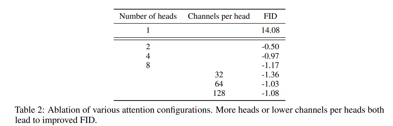
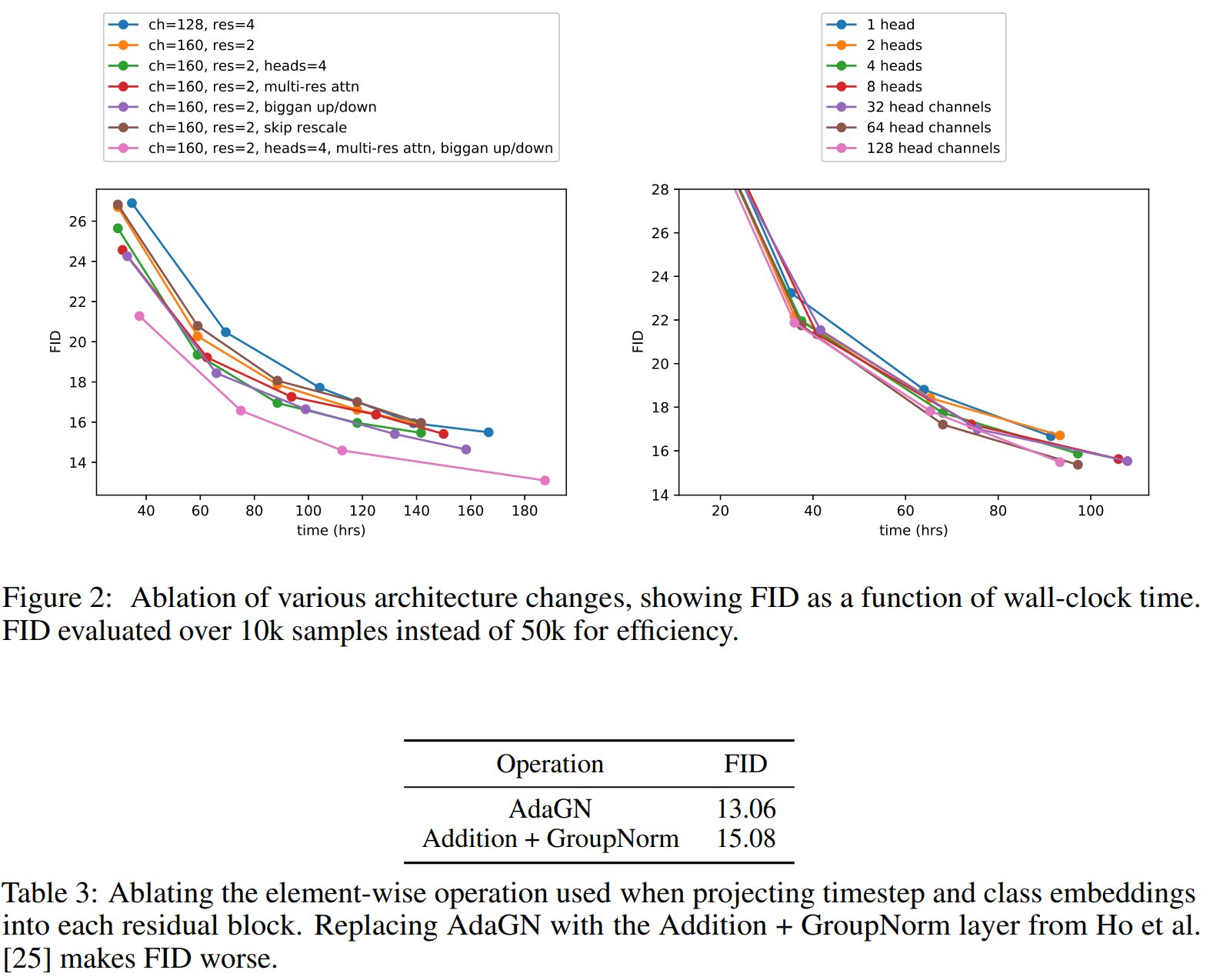
值得注意的是虽然增加模型深度可以改善效果,但是会增加训练时间,所以在接下来的实验没有使用这个措施。
表2 的结果显示使用更多的 heads 或者每个 head 使用更少的 channels 可以改善 FID,每个 head 使用 64 个 channels 的效果最佳。
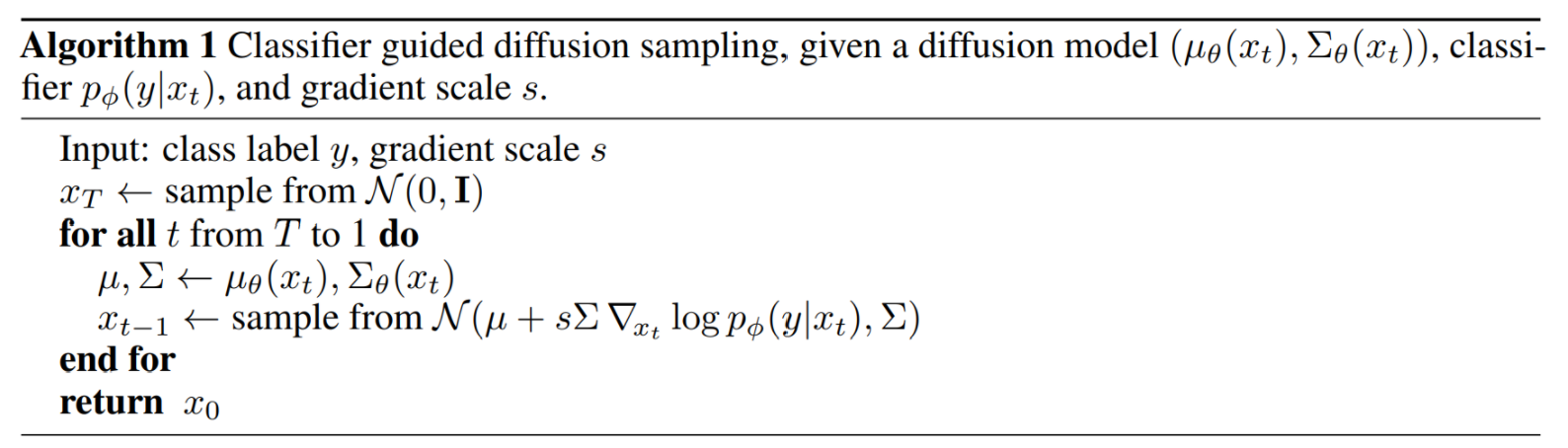
Adaptive Group Normalization
参考 adaptive group normalization (AdaGN),在group normalization 之后,将 timestep 和 class embedding 加进每个残差块:
\[\text{AdaGN}(h,y)=y_s \text{GroupNorm}(h)+y_b,\]式中,\(h\) 表示第一个卷积后的残差块的激活函数,\(y=[y_s,y_b]\) 是对 timestep 和 class embedding 的线性投影。
分类引导
除了将类别信息加进上节的 normalization layers 里, 文章还探索了增加一个classifier \(p(y\mid x)\) 来改进 diffusion generator,具体来说,对 noisy images \(x_t\) 训练一个分类器 \(p_{\phi}(y\mid x_t,t)\),然后用 \(\nabla_{x_t} \log p_{\phi}({x_t} \mid {y})\) 来指导 diffusion 生成类别为 \(y\) 的图像,具体做法分为如下 2 种情况:
stochastic diffusion sampling
以 label \(y\) 为条件时,使用如下方式采样:
\[\begin{aligned} p(x_t \mid x_{t+1},y) &= \frac{p(x_t,x_{t+1},y)}{p(x_{t+1},y)} \\ &= \frac{p(x_t,x_{t+1},y)}{p(y \mid x_{t+1})p(x_{t+1})} \\ &= \frac{p(x_t \mid x_{t+1})p(y \mid x_t,x_{t+1})p(x_{t+1})}{p(y \mid x_{t+1})p(x_{t+1})} \\ &= \frac{p(x_t \mid x_{t+1})p(y \mid x_t,x_{t+1})}{p(y \mid x_{t+1})} \\ &= \frac{p(x_t \mid x_{t+1})p(y \mid x_t)}{p(y \mid x_{t+1})} \\ \end{aligned},\]因为类别 \(y\) 的分布与 \(x_{t+1}\) 是独立的,所以:
\[\begin{aligned} p(y \mid x_t,x_{t+1}) &=p(x_{t+1} \mid x_t,y) \frac{p(y \mid x_t)}{p(x_{t+1}\mid x_t)}\\ &=p(x_{t+1} \mid x_t) \frac{p(y \mid x_t)}{p(x_{t+1}\mid x_t)}\\ &=p(y \mid x_t) \end{aligned}\]代入上式得:
\[\begin{aligned} p(x_t \mid x_{t+1},y) &= \frac{p(x_t \mid x_{t+1})p(y \mid x_t,x_{t+1})}{p(y \mid x_{t+1})} \\ &= \frac{p(x_t \mid x_{t+1})p(y \mid x_t)}{p(y \mid x_{t+1})} \\ \end{aligned},\]因为每个样本的 label 是已知的,所以 \(p(y \mid x_{t+1})\) 可视为常数,因此:
\[p_{\theta, \phi}\left(x_{t} \mid x_{t+1}, y\right)=Z\cdot p_{\theta}\left(x_{t} \mid x_{t+1}\right)\cdot p_{\phi}\left(y \mid x_{t}\right),\]式中, \(Z\) 是标准化常数,上式是 intractable 的,可以用 perturbed Gaussian distribution 近似。
(1) \(p_{\theta}\left(x_{t} \mid x_{t+1}\right)\) 项
我们的模型是使用高斯分布根据 \(x_{t+1}\) 预测 \(x_{t}\) :
\[\begin{aligned} p_{\theta}\left(x_{t} \mid x_{t+1}\right) &=\mathcal{N}(\mu, \Sigma) \\ \log p_{\theta}\left(x_{t} \mid x_{t+1}\right) &=-\frac{1}{2}\left(x_{t}-\mu\right)^{T} \Sigma^{-1}\left(x_{t}-\mu\right)+C \end{aligned}\](2) \(p_{\phi}\left(y \mid x_{t}\right)\) 项
在无限扩散时间步下, \(\|\Sigma\| \rightarrow 0\),可以假设 \(\log_{\phi} p(y\mid x_{t})\) 相比 \(\Sigma^{-1}\) 有着更低的曲率,那么我们可以对 \(\text{log} p_{\phi}(y \mid x_{t})\) 在 \(x_{t}=\mu\) 处进行泰勒展开:
\[\begin{aligned} \log p_{\phi}\left(y \mid x_{t}\right) &\left.\approx \log p_{\phi}\left(y \mid x_{t}\right)\right|_{x_{t}=\mu}+\left.\left(x_{t}-\mu\right) \nabla_{x_{t}} \log p_{\phi}\left(y \mid x_{t}\right)\right|_{x_{t}=\mu} \\ &=\left(x_{t}-\mu\right) g+C_{1} \end{aligned}\]式中,\(C_1\) 为常数,且:
\[g=\left. \nabla_{x_{t}} \log p_{\phi}\left(y \mid x_{t}\right)\right|_{x_{t}=\mu},\]综上:
\[\begin{aligned} \log \left(p_{\theta}\left(x_{t} \mid x_{t+1}\right) p_{\phi}\left(y \mid x_{t}\right)\right) & \approx-\frac{1}{2}\left(x_{t}-\mu\right)^{T} \Sigma^{-1}\left(x_{t}-\mu\right)+\left(x_{t}-\mu\right) g+C_{2} \\ &=-\frac{1}{2}\left(x_{t}-\mu-\Sigma g\right)^{T} \Sigma^{-1}\left(x_{t}-\mu-\Sigma g\right)+\frac{1}{2} g^{T} \Sigma g+C_{2} \\ &=-\frac{1}{2}\left(x_{t}-\mu-\Sigma g\right)^{T} \Sigma^{-1}\left(x_{t}-\mu-\Sigma g\right)+C_{3} \\ &=\log p(z)+C_{4}, z \sim \mathcal{N}(\mu+\Sigma g, \Sigma) \end{aligned},\]由上式可以看出条件转换运算类似于无条件运算使用 高斯分布近似,但是均值需要加上偏移量 \(\Sigma g\),具体的采样过程如下:
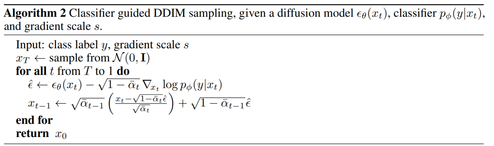
Conditional Sampling for DDIM
DDIM2 为确定性条件采样,不能用上面的采样方法。
根据贝叶斯公式:
\[p(\mathbf{x} \mid \mathbf{y}) = \frac{p(\mathbf{x}) p(\mathbf{y} \mid \mathbf{x}) }{p(\mathbf{y})},\]对上式两边同时求关于 \(\mathbf{x}\) 的导数,得到:
\[\nabla_\mathbf{x} \log p(\mathbf{x} \mid \mathbf{y}) = \nabla_\mathbf{x} \log p(\mathbf{x}) + \nabla_\mathbf{x} \log p(\mathbf{y} \mid \mathbf{x}),\]如果模型可以预测出添加到样本中的噪声 \(\epsilon_{\theta}\left(\mathbf{x_{t}}\right)\) , 可以得到:
\[\nabla_{\mathbf{x}_{t}} \log p_{\theta}\left(\mathbf{x}_{t}\right)=-\frac{1}{\sqrt{1-\bar{\alpha}_{t}}} \epsilon_{\theta}\left(\mathbf{x}_{t}\right),\]所以:
\[\begin{aligned} \nabla_\mathbf{x_t} \log p(\mathbf{x_t} \mid \mathbf{y}) &= \nabla_{\mathbf{x}_{t}} \log p_{\theta}\left(\mathbf{x}_{t}\right)+\nabla_{\mathbf{x}_{t}} \log p_{\phi}\left(\mathbf{y} \mid \mathbf{x}_{t}\right) \\ &= -\frac{1}{\sqrt{1-\bar{\alpha}_{t}}} \epsilon_{\theta}\left(\mathbf{x}_{t}\right)+\nabla_{x_{t}} \log p_{\phi}\left(\mathbf{y} \mid \mathbf{x}_{t}\right) \end{aligned},\]这样我们可以定义一个新的预测值 \(\hat{\epsilon}\left(\mathbf{x_{t}}\right)\) :
\[\hat{\epsilon}\left(\mathbf{x_{t}}\right):=\epsilon_{\theta}\left(\mathbf{x_{t}}\right)-\sqrt{1-\bar{\alpha}_{t}} \nabla_{\mathbf{x_{t}}} \log p_{\phi}\left(\mathbf{y} \mid \mathbf{x_{t}}\right),\]接下来可以使用 DDIM 的常规采样流程,只要将 \(\epsilon_{\theta}\left(\mathbf{x_{t}}\right)\) 替换成 \(\hat \epsilon_{\theta}\left(\mathbf{x_{t}}\right)\) ,具体做法如下:
Scaling Classifier Gradients
classifier 网络使用 UNet 模型的下采样部分, 在 8x8 特征层上使用 attention pool 产生最后的输出。
classifier 训练完后,就可以加进 diffusion 的采样过程生成样本。
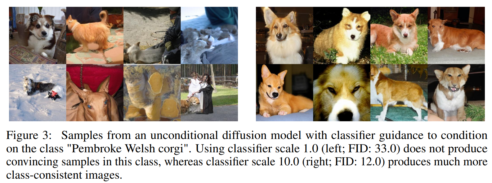
在实验中,作者发现需要对 classifier gradients 乘以一个大于1 的常数因子,如果因子为1,classifier 会赋予期望的类 50% 的概率生成最后的样本;如果提高 classifier gradients 因子,可以让 classifier 的类别概率提高到将近 100%,下图显示了这个效果。
缩放 classifier gradients 的影响
\[s\cdot \nabla_\mathbf{x} \log p(\mathbf{y} \mid \mathbf{x})=\nabla_\mathbf{x} \log \frac{1}{Z}p(\mathbf{y}\mid \mathbf{x})^s,\]式中,\(Z\) 为常数,当 \(s>1\) ,分布 \(p(\mathbf{y}\mid \mathbf{x})^s\) 比 \(p(\mathbf{y}\mid \mathbf{x})\) 更加陡峭,所以使用大的 gradient scale 会让模型更加关注 classifier ,从而产生更加逼真(多样性减少)的样本。
综上,得出本文最为重要的2点发现:
-
gradient scale 可以用于平衡图像生成的逼真度和多样性。
-
使用分类引导( classifier guidance)可以生成更加逼真的图像,基于这个观察,分类引导既可以用于生成 conditional 样本 \(p(x\mid y)\) 任务上,也可以用于生成 unconditional 样本 \(p(x)\) 任务上。
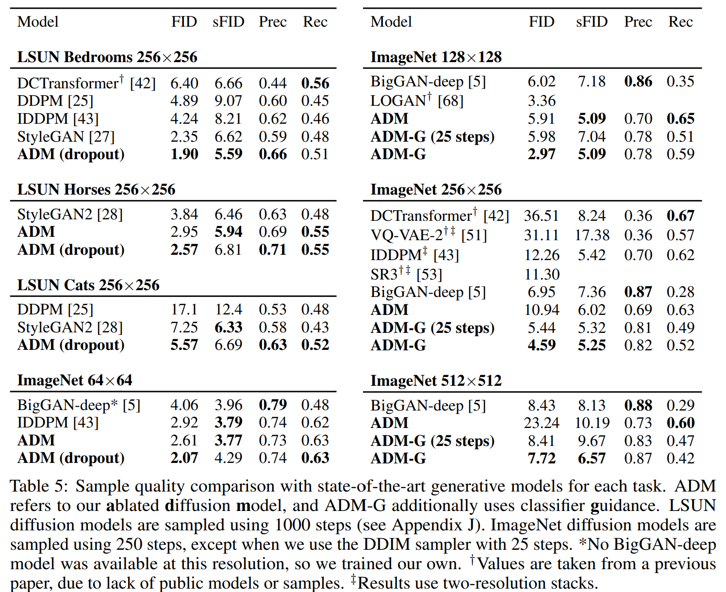
实验结果
guidance 影响
从表4结果来看,增加 classifier guidance 对于无条件和带条件的模型都可以提高样本生成质量,当 scale 足够高时,guided unconditional model 可以取得与 unguided conditional model 相近的 FID。
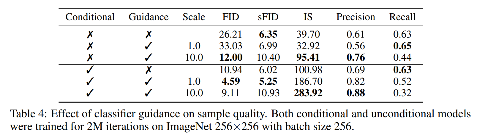
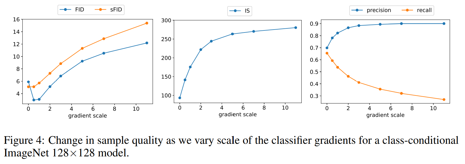
同时表4 还表明 classifier guidance 可以提高 precision(代价是降低 recall),所以其可以平衡样本多样性和逼真度,下图显示了 gradient scale 的影响,可以看出提高 gradient scale 可以平衡高精度的召回率(衡量多样性)以及 IS(衡量逼真度)。
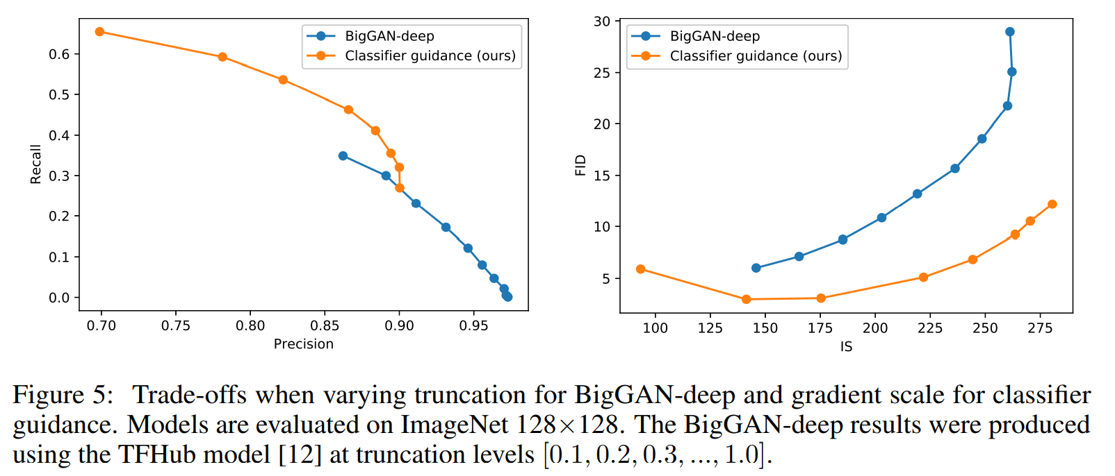
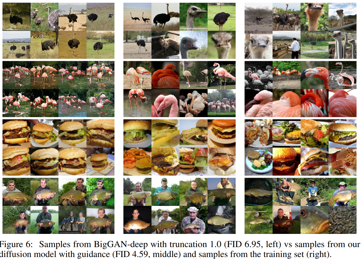
作者进一步对使用 guidance 的 diffusion 模型 和 BigGAN进行比较,发现2点有意思的现象:
- classifier guidance 在平衡 FID 和 IS 方面远好于 BigGAN ;
- classifier guidance 在达到一个 precision 阈值后,就无法取得更好的 precision。
结果
评估改进的模型架构在无条件图像生成的性能使用数据集 LSUN(bedroom, horse 和 cat),评估 classifier guidance 性能使用数据集 ImageNet (分辨率分别为 128×128, 256×256 和 512×512),几乎在每个任务上 diffusion models 都取得了 SOTA成绩。
代码分析
前向过程
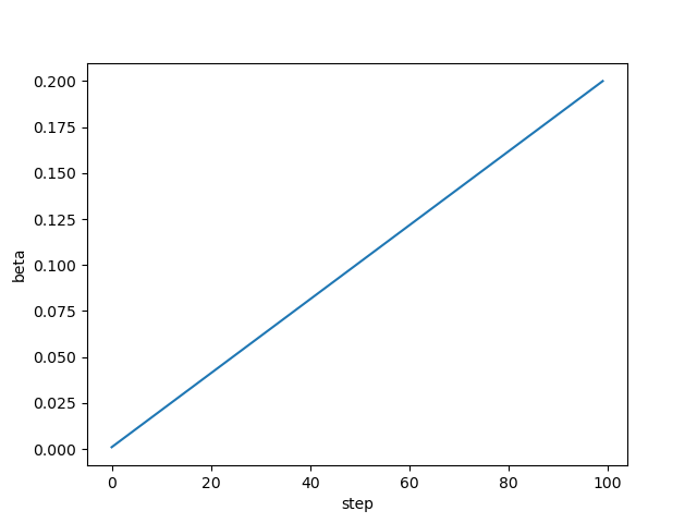
beta schedule
gaussian_diffusion. get_named_beta_schedule()
如果 num_diffusion_timesteps 设置为100,并且选用 linear schedule:
num_diffusion_timesteps=100
if schedule_name == "linear":
    scale = 1000 / num_diffusion_timesteps # scale: 10
    beta_start = scale * 0.0001  # beta_start: 0.001
    beta_end = scale * 0.02  # beta_end: 0.2
    betas= np.linspace(beta_start, beta_end, num_diffusion_timesteps, dtype=np.float64)
\(\beta\) 计算结果如下:
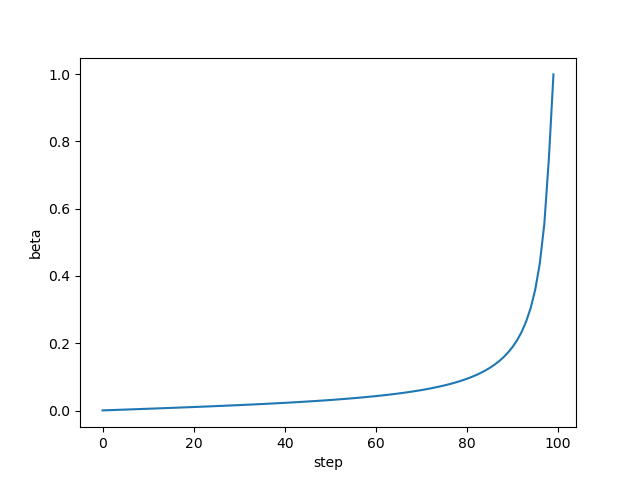
如果选用 linear schedule:
def betas_for_alpha_bar(num_diffusion_timesteps, alpha_bar, max_beta=0.999):
    """
    Create a beta schedule that discretizes the given alpha_t_bar function,
    which defines the cumulative product of (1-beta) over time from t = [0,1].

    :param num_diffusion_timesteps: the number of betas to produce.
    :param alpha_bar: a lambda that takes an argument t from 0 to 1 and
                      produces the cumulative product of (1-beta) up to that
                      part of the diffusion process.
    :param max_beta: the maximum beta to use; use values lower than 1 to
                     prevent singularities.
    """
    betas = []
    for i in range(num_diffusion_timesteps):
        t1 = i / num_diffusion_timesteps
        t2 = (i + 1) / num_diffusion_timesteps
        betas.append(min(1 - alpha_bar(t2) / alpha_bar(t1), max_beta))
    return np.array(betas)

if schedule_name == "cosine":
	betas_for_alpha_bar(num_diffusion_timesteps,
                    	lambda t: math.cos((t + 0.008) / 1.008 * math.pi / 2) ** 2)
\(\beta\) 计算结果如下:
参数计算
alphas: \(\alpha_t=1-\beta_t\)
alphas_cumprod: \(\bar \alpha_t = \prod_{i=1}^T \alpha_i\)
alphas_cumprod_prev: \(\bar \alpha_{t-1}\)
alphas_cumprod_next:\(\bar \alpha_{t+1}\)
sqrt_alphas_cumprod:\(\sqrt{\bar \alpha_t}\)
sqrt_one_minus_alphas_cumprod:\(\sqrt{1-\bar \alpha_t}\)
log_one_minus_alphas_cumprod:\(\log (1-\bar \alpha_t)\)
sqrt_recip_alphas_cumprod:\(\frac{1}{\sqrt{\bar \alpha_t}}\)
sqrt_recipm1_alphas_cumprod::\(\sqrt{\frac{1}{\bar \alpha_t}-1}\)
posterior_variance:\(\frac{\beta_t\cdot (1-\bar \alpha_{t-1})}{1-\bar \alpha_t}\)
posterior_mean_coef1:\(\frac{\beta_t\cdot \sqrt{\bar \alpha_{t-1}}}{1-\bar \alpha_t}\)
posterior_mean_coef2:\(\frac{(1-\bar \alpha_{t-1})\cdot \sqrt{\alpha_t}}{1-\bar \alpha_t}\)
# Use float64 for accuracy.
n_steps=100
betas=get_named_beta_schedule('linear', num_diffusion_timesteps=n_steps)
betas = np.array(betas, dtype=np.float64)
num_timesteps = int(betas.shape[0])

alphas = 1.0 - betas
alphas_cumprod = np.cumprod(alphas, axis=0)
alphas_cumprod_prev = np.append(1.0, alphas_cumprod[:-1])
alphas_cumprod_next = np.append(alphas_cumprod[1:], 0.0)

# calculations for diffusion q(x_t | x_{t-1}) and others
sqrt_alphas_cumprod = np.sqrt(alphas_cumprod)
sqrt_one_minus_alphas_cumprod = np.sqrt(1.0 - alphas_cumprod)
log_one_minus_alphas_cumprod = np.log(1.0 - alphas_cumprod)
sqrt_recip_alphas_cumprod = np.sqrt(1.0 / alphas_cumprod)
sqrt_recipm1_alphas_cumprod = np.sqrt(1.0 / alphas_cumprod - 1)

# calculations for posterior q(x_{t-1} | x_t, x_0)
posterior_variance = (betas * (1.0 - alphas_cumprod_prev) / (1.0 - alphas_cumprod))

# log calculation clipped because the posterior variance is 0 at the
# beginning of the diffusion chain.
posterior_log_variance_clipped = np.log(np.append(posterior_variance[1], posterior_variance[1:]))
posterior_mean_coef1 = (betas * np.sqrt(alphas_cumprod_prev) / (1.0 - alphas_cumprod))
posterior_mean_coef2 = ((1.0 - alphas_cumprod_prev)* np.sqrt(alphas)/ (1.0 - alphas_cumprod))
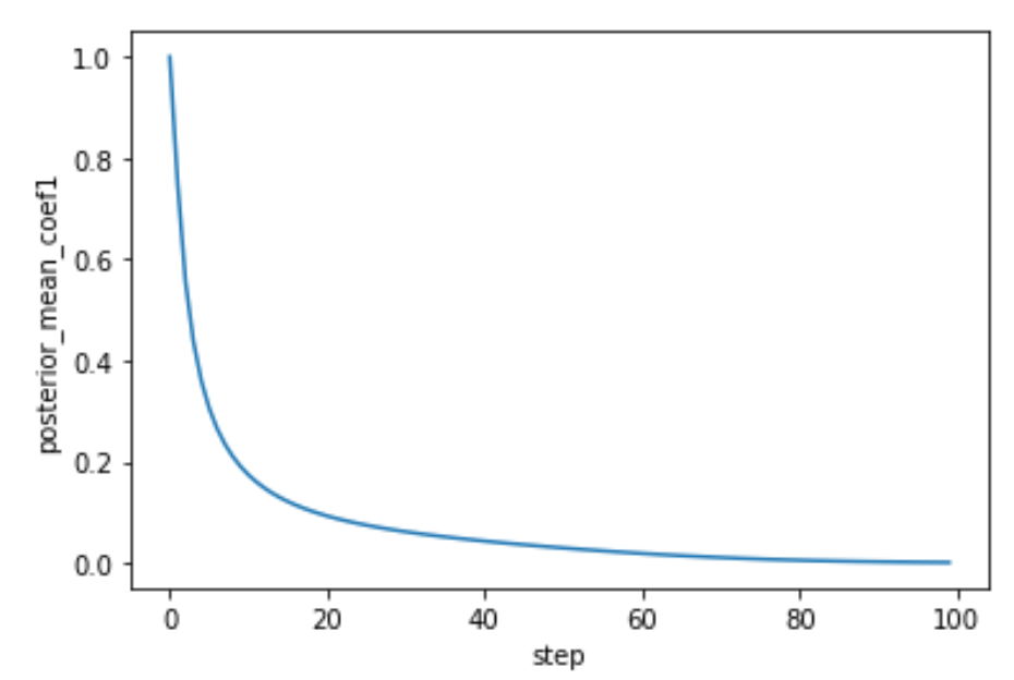
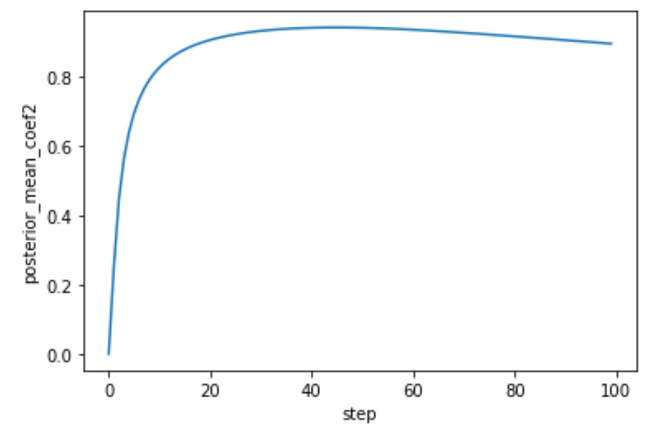
当使用 linear schedule 时,posterior_mean_coef1 和 posterior_mean_coef2 曲线如下:
正向过程
正向过程,根据 \(\mathbf{x_0}\) 计算 \(\mathbf{x_t}\):
\[q(\mathbf{x_t} \vert \mathbf{x_0}) = \mathcal{N}(\mathbf{x_t}; \sqrt{\bar{\alpha_t}} \mathbf{x_0}, (1 - \bar{\alpha_t})\mathbf{I}),\]这里涉及一个函数 _extract_into_tensor(), 其作用是将某个时间步的值的 shape 扩充成 broadcast_shape,例子:
某个 arr 值为 [1.00250941,1.57537666,6.38749852, 56.82470788,2.5753766] ,时间步为 3, 则对应的值为 56.82470788,因为后面需要代入公式计算,需要对形状进行扩展,比如需要扩展的形状为 (2, 3, 128, 128), 则通过 _extract_into_tensor 可以得到值全部为 56.82470788,形状为 (2, 3, 128, 128) 的 tensor。
def _extract_into_tensor(arr, timesteps, broadcast_shape):
    """
    Extract values from a 1-D numpy array for a batch of indices.

    :param arr: the 1-D numpy array.
    :param timesteps: a tensor of indices into the array to extract.
    :param broadcast_shape: a larger shape of K dimensions with the batch
                            dimension equal to the length of timesteps.
    :return: a tensor of shape [batch_size, 1, ...] where the shape has K dims.
    """
    res = th.from_numpy(arr).to(device=timesteps.device)[timesteps].float()
    while len(res.shape) < len(broadcast_shape):
        res = res[..., None]
    return res.expand(broadcast_shape)
arr=np.array([1.00250941,1.57537666,6.38749852, 56.82470788,2.5753766])
broadcast_shape=[2, 3, 128, 128]
timesteps=th.tensor([3, 3])
res=_extract_into_tensor(arr, timesteps, broadcast_shape)

print(res.shape)
print(th.unique(res))
输出结果:
torch.Size([2, 3, 128, 128])
tensor([56.8247])
接下来看函数 q_mean_variance() ,正向过程中的 mean 为 \(\sqrt{\bar{\alpha_t}} \mathbf{x_0}\) ,variance 为 \(1 - \bar{\alpha_t}\), 实现如下:
def q_mean_variance(self, x_start, t):
    """
        Get the distribution q(x_t | x_0).

        :param x_start: the [N x C x ...] tensor of noiseless inputs.
        :param t: the number of diffusion steps (minus 1). Here, 0 means one step.
        :return: A tuple (mean, variance, log_variance), all of x_start's shape.
        """
    mean = ( _extract_into_tensor(self.sqrt_alphas_cumprod, t, x_start.shape) * x_start)
    variance = _extract_into_tensor(1.0 - self.alphas_cumprod, t, x_start.shape)
    log_variance = _extract_into_tensor(self.log_one_minus_alphas_cumprod, t, x_start.shape)
    return mean, variance, log_variance
根据 \(q(\mathbf{x_t} \vert \mathbf{x_0})\) 可得:
\[\begin{aligned} \mathbf{x}_t = \sqrt{\bar{\alpha}_t}\mathbf{x_0} + \sqrt{1 - \bar{\alpha}_t}\mathbf{z} \\ \end{aligned},\]实现代码如下:
def q_sample(self, x_start, t, noise=None):
    """
        Diffuse the data for a given number of diffusion steps.

        In other words, sample from q(x_t | x_0).

        :param x_start: the initial data batch.
        :param t: the number of diffusion steps (minus 1). Here, 0 means one step.
        :param noise: if specified, the split-out normal noise.
        :return: A noisy version of x_start.
        """
    if noise is None:
        noise = th.randn_like(x_start)
        assert noise.shape == x_start.shape
        return (
            _extract_into_tensor(self.sqrt_alphas_cumprod, t, x_start.shape) * x_start
            + _extract_into_tensor(self.sqrt_one_minus_alphas_cumprod, t, x_start.shape)
            * noise
        )
反向过程
反向过程计算如下:
\[\mathbf{x_{t-1}} =\mu_{\theta}(\mathbf{x}_{t},t) + \sigma_{\theta}(\mathbf{x}_{t},t)\cdot \mathbf{z},\]需要分别计算 variance \(\sigma_{\theta}(\mathbf{x}_{t},t)\) 和 mean \(\mu_{\theta}(\mathbf{x}_{t},t)\) ,实现如下:
计算 variance
model_var_type 有2 种:ModelVarType.LEARNED 和 ModelVarType.LEARNED_RANGE。
如果 model_var_type 为 ModelVarType.LEARNED ,则:
model_log_variance = model_var_values
model_variance = th.exp(model_log_variance)
如果 model_var_type 为 ModelVarType.LEARNED_RANGE ,则:
min_log = _extract_into_tensor(self.posterior_log_variance_clipped, t, x.shape)
max_log = _extract_into_tensor(np.log(self.betas), t, x.shape)
# The model_var_values is [-1, 1] for [min_var, max_var].
frac = (model_var_values + 1) / 2
model_log_variance = frac * max_log + (1 - frac) * min_log
model_variance = th.exp(model_log_variance)
计算 mean
(1) 无条件
model_mean_type 有3种:ModelMeanType.PREVIOUS_X、ModelMeanType.START_X、ModelMeanType.EPSILON,
方法1: ModelMeanType.PREVIOUS_X
如果 model_mean_type 为 ModelMeanType.PREVIOUS_X ,计算:
\[\mu_{\theta}=\frac{1-\bar \alpha_t}{\beta_t\cdot \sqrt{\bar \alpha_{t-1}}}\cdot \mathbf{x_{t-1}}-\frac{(1-\bar \alpha_{t-1})\cdot \sqrt{\alpha_t}}{\beta_t\cdot \sqrt{\bar \alpha_{t-1}}}\mathbf{x_{t}},\]posterior_variance:\(\frac{\beta_t\cdot (1-\bar \alpha_{t-1})}{1-\bar \alpha_t}\)
posterior_mean_coef1:\(\frac{\beta_t\cdot \sqrt{\bar \alpha_{t-1}}}{1-\bar \alpha_t}\)
posterior_mean_coef2:\(\frac{(1-\bar \alpha_{t-1})\cdot \sqrt{\alpha_t}}{1-\bar \alpha_t}\)
def _predict_xstart_from_xprev(self, x_t, t, xprev):
    assert x_t.shape == xprev.shape
    return (  # (xprev - coef2*x_t) / coef1
        _extract_into_tensor(1.0 / self.posterior_mean_coef1, t, x_t.shape) * xprev
        - _extract_into_tensor(
            self.posterior_mean_coef2 / self.posterior_mean_coef1, t, x_t.shape
        )* x_t
    )
方法2: ModelMeanType.EPSILON
如果 model_mean_type 为 ModelMeanType.EPSILON,则使用 DDIM 计算的计算方法:
_predict_xstart_from_eps
因为 \(\mathbf{x}_t = \sqrt{\bar{\alpha}_t}\mathbf{x}_0 + \sqrt{1 - \bar{\alpha}_t}\mathbf{\epsilon}\) ,可以根据 \(\mathbf{x}_t\) 预测 \(\mathbf{x}_0\):
\[\mathbf{x}_0= \frac{1}{\sqrt{\bar \alpha_t}}\mathbf{x}_t- \sqrt{\frac{1}{\bar \alpha_t}-1}\cdot\mathbf{\epsilon}_{\theta}^{(t)}(\mathbf{x}_t),\]sqrt_recip_alphas_cumprod:\(\frac{1}{\sqrt{\bar \alpha_t}}\)
sqrt_recipm1_alphas_cumprod:\(\sqrt{\frac{1}{\bar \alpha_t}-1}\)
def _predict_xstart_from_eps(self, x_t, t, eps):
    assert x_t.shape == eps.shape
    return (
        _extract_into_tensor(self.sqrt_recip_alphas_cumprod, t, x_t.shape) * x_t
        - _extract_into_tensor(self.sqrt_recipm1_alphas_cumprod, t, x_t.shape) * eps
    )
然后根据 \(\mathbf{x}_{t}\) 和 \(\mathbf{x}_{0}\) ,通过 \(q\left(\mathbf{x}_{t-1} \mid \mathbf{x}_{t}, \mathbf{x}_{0}\right)\) 计算 \(\mathbf{x}_{t-1}\) , 得到 model_mean:
\[\mu_{\theta}=\frac{\sqrt{\bar{\alpha}_{t-1}} \beta_{t}}{1-\bar{\alpha}_{t}} \mathbf{x}_{0}+\frac{\sqrt{\alpha_{\iota}}\left(1-\bar{\alpha}_{ t-1}\right)}{1-\bar{\alpha}_{t}} \mathbf{x}_{t},\]根据 1.2 节中的参数计算:
posterior_mean_coef1:\(\frac{\beta_t\cdot \sqrt{\bar \alpha_{t-1}}}{1-\bar \alpha_t}\)
posterior_mean_coef2:\(\frac{(1-\bar \alpha_{t-1})\cdot \sqrt{\alpha_t}}{1-\bar \alpha_t}\)
posterior_variance:\(\frac{1-\bar \alpha_{t-1}}{1-\bar \alpha_t}\cdot \beta_t\)
实现代码如下:
def q_posterior_mean_variance(self, x_start, x_t, t):
    """
        Compute the mean and variance of the diffusion posterior:

            q(x_{t-1} | x_t, x_0)

        """
    assert x_start.shape == x_t.shape
    posterior_mean = (
        _extract_into_tensor(self.posterior_mean_coef1, t, x_t.shape) * x_start
        + _extract_into_tensor(self.posterior_mean_coef2, t, x_t.shape) * x_t
    )
    posterior_variance = _extract_into_tensor(self.posterior_variance, t, x_t.shape)
    posterior_log_variance_clipped = _extract_into_tensor(
        self.posterior_log_variance_clipped, t, x_t.shape
    )
    assert (
        posterior_mean.shape[0]
        == posterior_variance.shape[0]
        == posterior_log_variance_clipped.shape[0]
        == x_start.shape[0]
    )
    return posterior_mean, posterior_variance, posterior_log_variance_clipped
variance 和 mean 计算完整的实现代码如下:
def p_mean_variance(self, model, x, t, clip_denoised=True, denoised_fn=None, model_kwargs=None):
    """
        Apply the model to get p(x_{t-1} | x_t), as well as a prediction of
        the initial x, x_0.

        :param model: the model, which takes a signal and a batch of timesteps
                      as input.
        :param x: the [N x C x ...] tensor at time t.
        :param t: a 1-D Tensor of timesteps.
        :param clip_denoised: if True, clip the denoised signal into [-1, 1].
        :param denoised_fn: if not None, a function which applies to the
            x_start prediction before it is used to sample. Applies before
            clip_denoised.
        :param model_kwargs: if not None, a dict of extra keyword arguments to
            pass to the model. This can be used for conditioning.
        :return: a dict with the following keys:
                 - 'mean': the model mean output.
                 - 'variance': the model variance output.
                 - 'log_variance': the log of 'variance'.
                 - 'pred_xstart': the prediction for x_0.
        """
    if model_kwargs is None:
        model_kwargs = {}

        B, C = x.shape[:2]
        assert t.shape == (B,)
        model_output = model(x, self._scale_timesteps(t), **model_kwargs)

        #-------------------------------#
        #             variance
        #-------------------------------#
        if self.model_var_type in [ModelVarType.LEARNED, ModelVarType.LEARNED_RANGE]:
            assert model_output.shape == (B, C * 2, *x.shape[2:])

            model_output, model_var_values = th.split(model_output, C, dim=1)

            if self.model_var_type == ModelVarType.LEARNED:
                model_log_variance = model_var_values
                model_variance = th.exp(model_log_variance)

            else:
                min_log = _extract_into_tensor(self.posterior_log_variance_clipped, t, x.shape)
                max_log = _extract_into_tensor(np.log(self.betas), t, x.shape)
                # The model_var_values is [-1, 1] for [min_var, max_var].
                frac = (model_var_values + 1) / 2
                model_log_variance = frac * max_log + (1 - frac) * min_log
                model_variance = th.exp(model_log_variance)

        else:
            model_variance, model_log_variance = {
                # for fixedlarge, we set the initial (log-)variance like so
                # to get a better decoder log likelihood.
                ModelVarType.FIXED_LARGE: (
                    np.append(self.posterior_variance[1], self.betas[1:]),
                    np.log(np.append(self.posterior_variance[1], self.betas[1:])),
                ),
                ModelVarType.FIXED_SMALL: (
                    self.posterior_variance,
                    self.posterior_log_variance_clipped,
                ),
            }[self.model_var_type]
            model_variance = _extract_into_tensor(model_variance, t, x.shape)
            model_log_variance = _extract_into_tensor(model_log_variance, t, x.shape)


        #-------------------------------#
        #              mean
        #-------------------------------#
        def process_xstart(x):
            if denoised_fn is not None:
                x = denoised_fn(x)
                if clip_denoised:
                    return x.clamp(-1, 1)
                return x

        if self.model_mean_type == ModelMeanType.PREVIOUS_X:
            pred_xstart = process_xstart(
                self._predict_xstart_from_xprev(x_t=x, t=t, xprev=model_output))
            model_mean = model_output

        elif self.model_mean_type in [ModelMeanType.START_X, ModelMeanType.EPSILON]:
            if self.model_mean_type == ModelMeanType.START_X:
                pred_xstart = process_xstart(model_output)
            else:
                pred_xstart = process_xstart(self._predict_xstart_from_eps(x_t=x, t=t, eps=model_output))
                model_mean, _, _ = self.q_posterior_mean_variance(x_start=pred_xstart, x_t=x, t=t)

        else:
            raise NotImplementedError(self.model_mean_type)

        assert (
             model_mean.shape == model_log_variance.shape == pred_xstart.shape == x.shape)

        return {
            "mean": model_mean,
            "variance": model_variance,
            "log_variance": model_log_variance,
            "pred_xstart": pred_xstart,
          }
(2) 有条件
(1) condition_mean 方法
当带条件时,需要在无条件 mean 基础上加上偏移量,采样过程如下:
\(\nabla_{\mathbf{x_{t}}} \log p_{\phi}\left(\mathbf{y} \mid \mathbf{x_{t}}\right)\) 计算代码如下:
def cond_fn(x, t, y=None):
    assert y is not None
    with th.enable_grad():
        x_in = x.detach().requires_grad_(True)
        logits = classifier(x_in, t)
        log_probs = F.log_softmax(logits, dim=-1)
        selected = log_probs[range(len(logits)), y.view(-1)]
        return th.autograd.grad(selected.sum(), x_in)[0] * args.classifier_scale
如何理解 \(\log p_{\phi}\left(\mathbf{y} \mid \mathbf{x_{t}}\right)\)?
计算 \(\log p_{\phi}\left(\mathbf{y} \mid \mathbf{x_{t}}\right)\) 部分的计算代码如下:
log_probs = F.log_softmax(logits, dim=-1)
selected = log_probs[range(len(logits)), y.view(-1)]
selected.sum()
上面的计算过程其实就是 cross_entropy,只是相差了系数和负号,可以做个比较:
import torch
import torch.nn as nn
import torch.nn.functional as F

num_calsses=1000
y=torch.tensor([2,10])
logits=torch.randn((2,num_calsses))

## log p(y|x)
log_probs = F.log_softmax(logits, dim=-1)
selected = log_probs[range(len(logits)), y.view(-1)]
res=selected.sum()
print(res)

## cross_entropy(x,y)
res=F.cross_entropy(logits,y)
print(res)
结果为:
log p(y|x):    tensor(-17.0620)
cross_entropy: tensor(8.5310)s
cross_entropy 取了均值,所以相差一个系数 2和负号,所以 \(\log p_{\phi}\left(\mathbf{y} \mid \mathbf{x_{t}}\right)\) 衡量了 \(\mathbf{x_{t}}\) 与 \(\mathbf{y}\) 的距离,两者关系如下:
\[\log p_{\phi}\left(\mathbf{y} \mid \mathbf{x_{t}}\right)=-N\cdot \text{CrossEntropy}(\mathbf{x_{t}},\mathbf{y}),\]所以带条件的 mean 更新本质上就是使用的 SGD 梯度下降法:
\[\begin{aligned} \mathbf{\mu_{t-1}} &=\mu_t+s\Sigma\cdot \nabla_{\mathbf{x_{t}}} \log p_{\phi}\left(\mathbf{y} \mid \mathbf{x_{t}}\right)\\ &=\mathbf{\mu_{t}}-\alpha \nabla_{J_{\phi}}(\mathbf{x_{t}},\mathbf{y}) \end{aligned},\]\(\mathbf{\mu_{t-1}}\) 的更新代码如下:
def condition_mean(self, cond_fn, p_mean_var, x, t, model_kwargs=None):
    """
    Compute the mean for the previous step, given a function cond_fn that
    computes the gradient of a conditional log probability with respect to
    x. In particular, cond_fn computes grad(log(p(y|x))), and we want to
    condition on y.

    This uses the conditioning strategy from Sohl-Dickstein et al. (2015).
    """
    gradient = cond_fn(x, self._scale_timesteps(t), **model_kwargs)
    new_mean = (
        p_mean_var["mean"].float() + p_mean_var["variance"] * gradient.float()
    )
    return new_mean
(2) condition_score 方法
代码如下:
def condition_score(self, cond_fn, p_mean_var, x, t, model_kwargs=None):
    """
    Compute what the p_mean_variance output would have been, should the
    model's score function be conditioned by cond_fn.

    See condition_mean() for details on cond_fn.

    Unlike condition_mean(), this instead uses the conditioning strategy
    from Song et al (2020).
    """
    alpha_bar = _extract_into_tensor(self.alphas_cumprod, t, x.shape)

    eps = self._predict_eps_from_xstart(x, t, p_mean_var["pred_xstart"])
    eps = eps - (1 - alpha_bar).sqrt() * cond_fn(
        x, self._scale_timesteps(t), **model_kwargs
    )

    out = p_mean_var.copy()
    out["pred_xstart"] = self._predict_xstart_from_eps(x, t, eps)
    out["mean"], _, _ = self.q_posterior_mean_variance(
        x_start=out["pred_xstart"], x_t=x, t=t
    )
    return out
生成样本
def p_sample(
    self,
    model,
    x,
    t,
    clip_denoised=True,
    denoised_fn=None,
    cond_fn=None,
    model_kwargs=None,
):
    """
    Sample x_{t-1} from the model at the given timestep.

    :param model: the model to sample from.
    :param x: the current tensor at x_{t-1}.
    :param t: the value of t, starting at 0 for the first diffusion step.
    :param clip_denoised: if True, clip the x_start prediction to [-1, 1].
    :param denoised_fn: if not None, a function which applies to the
        x_start prediction before it is used to sample.
    :param cond_fn: if not None, this is a gradient function that acts
                    similarly to the model.
    :param model_kwargs: if not None, a dict of extra keyword arguments to
        pass to the model. This can be used for conditioning.
    :return: a dict containing the following keys:
             - 'sample': a random sample from the model.
             - 'pred_xstart': a prediction of x_0.
    """
    out = self.p_mean_variance(
        model,
        x,
        t,
        clip_denoised=clip_denoised,
        denoised_fn=denoised_fn,
        model_kwargs=model_kwargs,
    )
    noise = th.randn_like(x)
    nonzero_mask = (
        (t != 0).float().view(-1, *([1] * (len(x.shape) - 1)))
    )  # no noise when t == 0
    if cond_fn is not None:
        out["mean"] = self.condition_mean(
            cond_fn, out, x, t, model_kwargs=model_kwargs
        )
    sample = out["mean"] + nonzero_mask * th.exp(0.5 * out["log_variance"]) * noise
    return {"sample": sample, "pred_xstart": out["pred_xstart"]}
参考
-
Prafulla Dhariwal, Alex Nichol, “Diffusion Models Beat GANs on Image Synthesis”, Computer Vision and Pattern Recognition, 2021. code ↩