This summer, I’m interning at Spotify in New York City, where I’m working on content-based music recommendation using convolutional neural networks. In this post, I’ll explain my approach and show some preliminary results.
Overview
This is going to be a long post, so here’s an overview of the different sections. If you want to skip ahead, just click the section title to go there.
- Collaborative filtering
A very brief introduction, its virtues and its flaws. - Content-based recommendation
What to do when no usage data is available. - Predicting listening preferences with deep learning
Music recommendation based on audio signals. - Scaling up
Some details about the convnets I’ve been training at Spotify. - Analysis: what is it learning?
A look at what the convnets learn about music, with lots of audio examples, yay! - What will this be used for?
Some potential applications of my work. - Future work
- Conclusion
Collaborative filtering
Traditionally, Spotify has relied mostly on collaborative filtering approaches to power their recommendations. The idea of collaborative filtering is to determine the users’ preferences from historical usage data. For example, if two users listen to largely the same set of songs, their tastes are probably similar. Conversely, if two songs are listened to by the same group of users, they probably sound similar. This kind of information can be exploited to make recommendations.
Pure collaborative filtering approaches do not use any kind of information about the items that are being recommended, except for the consumption patterns associated with them: they are content-agnostic. This makes these approaches widely applicable: the same type of model can be used to recommend books, movies or music, for example.
Unfortunately, this also turns out to be their biggest flaw. Because of their reliance on usage data, popular items will be much easier to recommend than unpopular items, as there is more usage data available for them. This is usually the opposite of what we want. For the same reason, the recommendations can often be rather boring and predictable.
Another issue that is more specific to music, is the heterogeneity of content with similar usage patterns. For example, users may listen to entire albums in one go, but albums may contain intro tracks, outro tracks, interludes, cover songs and remixes. These items are atypical for the artist in question, so they aren’t good recommendations. Collaborative filtering algorithms will not pick up on this.
But perhaps the biggest problem is that new and unpopular songs cannot be recommended: if there is no usage data to analyze, the collaborative filtering approach breaks down. This is the so-called cold-start problem. We want to be able to recommend new music right when it is released, and we want to tell listeners about awesome bands they have never heard of. To achieve these goals, we will need to use a different approach.
Content-based recommendation
Recently, Spotify has shown considerable interest in incorporating other sources of information into their recommendation pipeline to mitigate some of these problems, as evidenced by their acquisition of music intelligence platform company The Echo Nest a few months back. There are many different kinds of information associated with music that could aid recommendation: tags, artist and album information, lyrics, text mined from the web (reviews, interviews, …), and the audio signal itself.
Of all these information sources, the audio signal is probably the most difficult to use effectively. There is quite a large semantic gap between music audio on the one hand, and the various aspects of music that affect listener preferences on the other hand. Some of these are fairly easy to extract from audio signals, such as the genre of the music and the instruments used. Others are a little more challenging, such as the mood of the music, and the year (or time period) of release. A couple are practically impossible to obtain from audio: the geographical location of the artist and lyrical themes, for example.
Despite all these challenges, it is clear that the actual sound of a song will play a very big role in determining whether or not you enjoy listening to it - so it seems like a good idea to try to predict who will enjoy a song by analyzing the audio signal.
Predicting listening preferences with deep learning
In December last year, my colleague Aäron van den Oord and I published a paper on this topic at NIPS, titled ‘Deep content-based music recommendation‘. We tried to tackle the problem of predicting listening preferences from audio signals by training a regression model to predict the latent representations of songs that were obtained from a collaborative filtering model. This way, we could predict the representation of a song in the collaborative filtering space, even if no usage data was available. (As you can probably infer from the title of the paper, the regression model in question was a deep neural network.)
The underlying idea of this approach is that many collaborative filtering models work by projecting both the listeners and the songs into a shared low-dimensional latent space. The position of a song in this space encodes all kinds of information that affects listening preferences. If two songs are close together in this space, they are probably similar. If a song is close to a user, it is probably a good recommendation for that user (provided that they haven’t heard it yet). If we can predict the position of a song in this space from audio, we can recommend it to the right audience without having to rely on historical usage data.
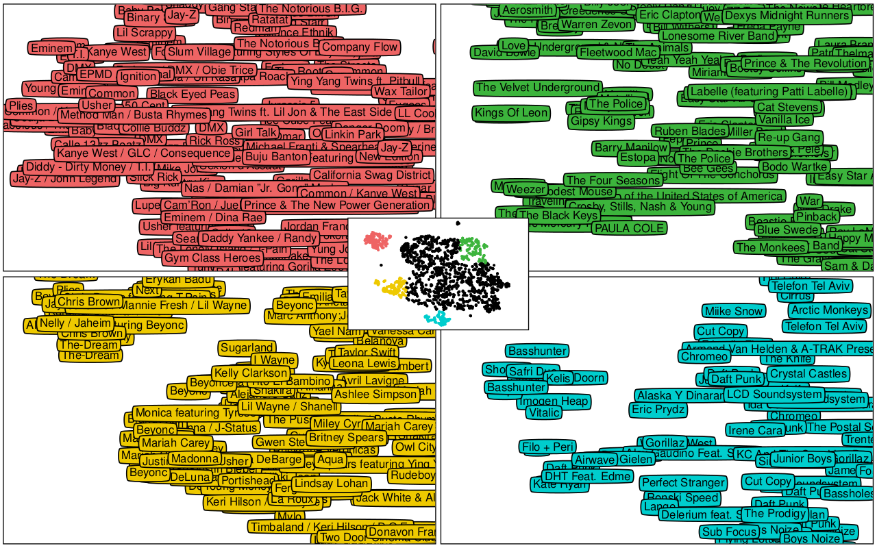
We visualized this in the paper by projecting the predictions of our model in the latent space down to two dimensions using the t-SNE algorithm. As you can see below on the resulting map, similar songs cluster together. Rap music can be found mostly in the top left corner, whereas electronic artists congregate at the bottom of the map.
Scaling up
The deep neural network that we trained for the paper consisted of two convolutional layers and two fully connected layers. The input consisted of spectrograms of 3 second fragments of audio. To get a prediction for a longer clip, we just split it up into 3 second windows and averaged the predictions across these windows.
At Spotify, I have access to a larger dataset of songs, and a bunch of different latent factor representations obtained from various collaborative filtering models. They also got me a nice GPU to run my experiments on. This has allowed me to scale things up quite a bit. I am currently training convolutional neural networks (convnets) with 7 or 8 layers in total, using much larger intermediate representations and many more parameters.
Architecture
Below is an example of an architecture that I’ve tried out, which I will describe in more detail. It has four convolutional layers and three dense layers. As you will see, there are some important differences between convnets designed for audio signals and their more traditional counterparts used for computer vision tasks.
Warning: gory details ahead! Feel free to skip ahead to ‘Analysis’ if you don’t care about things like ReLUs, max-pooling and minibatch gradient descent.
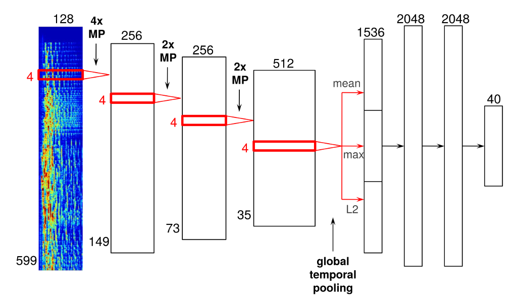
The input to the network consists of mel-spectrograms, with 599 frames and 128 frequency bins. A mel-spectrograms is a kind of time-frequency representation. It is obtained from an audio signal by computing the Fourier transforms of short, overlapping windows. Each of these Fourier transforms constitutes a frame. These successive frames are then concatenated into a matrix to form the spectrogram. Finally, the frequency axis is changed from a linear scale to a mel scale to reduce the dimensionality, and the magnitudes are scaled logarithmically.
The convolutional layers are displayed as red rectangles delineating the shape of the filters that slide across their inputs. They have rectified linear units (ReLUs, with activation function max(0, x)). Note that all these convolutions are one-dimensional; the convolution happens only in the time dimension, not in the frequency dimension. Although it is technically possible to convolve along both axes of the spectrogram, I am not currently doing this. It is important to realize that the two axes of a spectrogram have different meanings (time vs. frequency), which is not the case for images. As a result, it doesn’t really make sense to use square filters, which is what is typically done in convnets for image data.
Between the convolutional layers, there are max-pooling operations to downsample the intermediate representations in time, and to add some time invariance in the process. These are indicated with ‘MP’. As you can see I used a filter size of 4 frames in every convolutional layer, with max-pooling with a pool size of 4 between the first and second convolutional layers (mainly for performance reasons), and with a pool size of 2 between the other layers.
After the last convolutional layer, I added a global temporal pooling layer. This layer pools across the entire time axis, effectively computing statistics of the learned features across time. I included three different pooling functions: the mean, the maximum and the L2-norm.
I did this because the absolute location of features detected in the audio signal is not particularly relevant for the task at hand. This is not the case in image classification: in an image, it can be useful to know roughly where a particular feature was detected. For example, a feature detecting clouds would be more likely to activate for the top half of an image. If it activates in the bottom half, maybe it is actually detecting a sheep instead. For music recommendation, we are typically only interested in the overall presence or absence of certain features in the music, so it makes sense to perform pooling across time.
Another way to approach this problem would be to train the network on short audio fragments, and average the outputs across windows for longer fragments, as we did in the NIPS paper. However, incorporating the pooling into the model seems like a better idea, because it allows for this step to be taken into account during learning.
The globally pooled features are fed into a series of fully-connected layers with 2048 rectified linear units. In this network, I have two of them. The last layer of the network is the output layer, which predicts 40 latent factors obtained from the vector_exp algorithm, one of the various collaborative filtering algorithms that are used at Spotify.
Training
The network is trained to minimize the mean squared error (MSE) between the latent factor vectors from the collaborative filtering model and the predictions from audio. These vectors are first normalized so they have a unit norm. This is done to reduce the influence of song popularity (the norms of latent factor vectors tend to be correlated with song popularity for many collaborative filtering models). Dropout is used in the dense layers for regularization.
The dataset I am currently using consists of mel-spectrograms of 30 second excerpts extracted from the middle of the 1 million most popular tracks on Spotify. I am using about half of these for training (0.5M), about 5000 for online validation, and the remainder for testing. During training, the data is augmented by slightly cropping the spectrograms along the time axis with a random offset.
The network is implemented in Theano, and trained using minibatch gradient descent with Nesterov momentum on a NVIDIA GeForce GTX 780Ti GPU. Data loading and augmentation happens in a separate process, so while the GPU is training on a chunk of data, the next one can be loaded in parallel. About 750000 gradient updates are performed in total. I don’t remember exactly how long this particular architecture took to train, but all of the ones I’ve tried have taken between 18 and 36 hours.
Variations
As I mentioned before, this is just one example of an architecture that I’ve tried. Some other things I have tried / will try include:
- More layers!
- Using maxout units instead of rectified linear units.
- Using stochastic pooling instead of max-pooling.
- Incorporating L2 normalization into the output layer of the network.
- Data augmentation by stretching or compressing the spectrograms across time.
- Concatenating multiple latent factor vectors obtained from different collaborative filtering models.
Here are some things that didn’t work quite as well as I’d hoped:
- Adding ‘bypass’ connections from all convolutional layers to the fully connected part of the network, with global temporal pooling in between. The underlying assumption was that statistics about low-level features could also be useful for recommendation, but unfortunately this hampered learning too much.
- Predicting the conditional variance of the factors as in mixture density networks, to get confidence estimates for the predictions and to identify songs for which latent factor prediction is difficult. Unfortunately this seemed to make training quite a lot harder, and the resulting confidence estimates did not behave as expected.
Analysis: what is it learning?
Now for the cool part: what are these networks learning? What do the features look like? The main reason I chose to tackle this problem with convnets, is because I believe that music recommendation from audio signals is a pretty complex problem bridging many levels of abstraction. My hope was that successive layers of the network would learn progressively more complex and invariant features, as they do for image classification problems.
It looks like that’s exactly what is happening. First, let’s take a look at the first convolutional layer, which learns a set of filters that are applied directly to the input spectrograms. These filters are easy to visualize. They are shown in the image below. Click for a high resolution version (5584x562, ~600kB). Negative values are red, positive values are blue and white is zero. Note that each filter is only four frames wide. The individual filters are separated by dark red vertical lines.

From this representation, we can see that a lot of the filters pick up harmonic content, which manifests itself as parallel red and blue bands at different frequencies. Sometimes, these bands are are slanted up or down, indicating the presence of rising and falling pitches. It turns out that these filters tend to detect human voices.
Playlists for low-level features: maximal activation
To get a better idea of what the filters learn, I made some playlists with songs from the test set that maximally activate them. Below are a few examples. There are 256 filters in the first layer of the network, which I numbered from 0 to 255. Note that this numbering is arbitrary, as they are unordered.
These four playlists were obtained by finding songs that maximally activate a given filter in the 30 seconds that were analyzed. I selected a few interesting looking filters from the first convolutional layer and computed the feature representations for each of these, and then searched for the maximal activations across the entire test set. Note that you should listen to the middle of the tracks to hear what the filters are picking up on, as this is the part of the audio signal that was analyzed.
All of the Spotify playlists below should have 10 tracks. Some of them may not be available in all countries due to licensing issues.
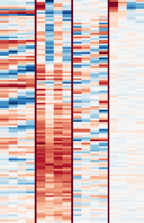
- Filter 14 seems to pick up vibrato singing.
- Filter 242 picks up some kind of ringing ambience.
- Filter 250 picks up vocal thirds, i.e. multiple singers singing the same thing, but the notes are a major third (4 semitones) apart.
- Filter 253 picks up various types of bass drum sounds.
The genres of the tracks in these playlists are quite varied, which indicates that these features are picking up mainly low-level properties of the audio signals.
Playlists for low-level features: average activation
The next four playlists were obtained in a slightly different way: I computed the average activation of each feature across time for each track, and then found the maximum across those. This means that for these playlists, the filter in question is constantly active in the 30 seconds that were analyzed (i.e. it’s not just one ‘peak’). This is more useful for detecting harmonic patterns.
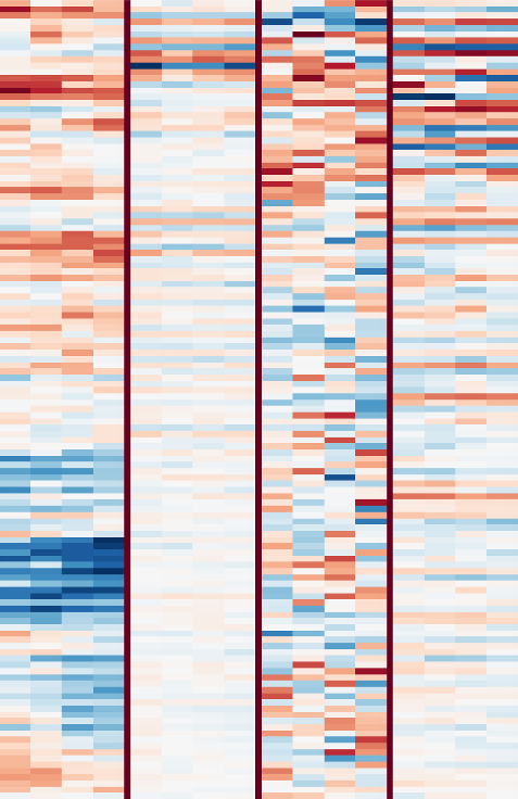
- Filter 1 picks up noise and (guitar) distortion.
- Filter 2 seems to pick up a specific pitch: a low Bb. It also picks up A sometimes (a semitone below) because the frequency resolution of the mel-spectrograms is not high enough to distinguish them.
- Filter 4 picks up various low-pitched drones.
- Filter 28 picks up the A chord. It seems to pick up both the minor and major versions, so it might just be detecting the pitches A and E (the fifth).
I thought it was very interesting that the network is learning to detect specific pitches and chords. I had previously assumed that the exact pitches or chords occurring in a song would not really affect listener preference. I have two hypotheses for why this might be happening:
- The network is just learning to detect harmonicity, by learning various filters for different kinds of harmonics. These are then pooled together at a higher level to detect harmonicity across different pitches.
- The network is learning that some chords and chord progressions are more common than others in certain genres of music.
I have not tried to verify either of these, but it seems like the latter would be pretty challenging for the network to pick up on, so I think the former is more likely.
Playlists for high-level features
Each layer in the network takes the feature representation from the layer below, and extracts a set of higher-level features from it. At the topmost fully-connected layer of the network, just before the output layer, the learned filters turn out to be very selective for certain subgenres. For obvious reasons, it is non-trivial to visualize what these filters pick up on at the spectrogram level. Below are six playlists with songs from the test set that maximally activate some of these high-level filters.
It is clear that each of these filters is identifying specific genres. Interestingly some filters, like #15 for example, seem to be multimodal: they activate strongly for two or more styles of music, and those styles are often completely unrelated. Presumably the output of these filters is disambiguated when viewed in combination with the activations of all other filters.
Filter 37 is interesting because it almost seems like it is identifying the Chinese language. This is not entirely impossible, since the phoneme inventory of Chinese is quite distinct from other languages. A few other seemingly language-specific filters seem to be learned: there is one that detects rap music in Spanish, for example. Another possibility is that Chinese pop music has some other characteristic that sets it apart, and the model is picking up on that instead.
I spent some time analyzing the first 50 or so filters in detail. Some other filter descriptions I came up with are: lounge, reggae, darkwave, country, metalcore, salsa, Dutch and German carnival music, children’s songs, dance, vocal trance, punk, Turkish pop, and my favorite, ‘exclusively Armin van Buuren’. Apparently he has so many tracks that he gets his own filter.
The filters learned by Alex Krizhevsky’s ImageNet network have been reused for various other computer vision tasks with great success. Based on their diversity and invariance properties, it seems that these filters learned from audio signals may also be useful for other music information retrieval tasks besides predicting latent factors.
Similarity-based playlists
Predicted latent factor vectors can be used to find songs that sound similar. Below are a couple of playlists that were generated by predicting the factor vector for a given song, and then finding other songs in the test set whose predicted factor vectors are close to it in terms of cosine distance. As a result, the first track in the playlist is always the query track itself.
Most of the similar tracks are pretty decent recommendations for fans of the query tracks. Of course these lists are far from perfect, but considering that they were obtained based only on the audio signals, the results are pretty decent. One example where things go wrong is the list for ‘My Favorite Things’ by John Coltrane, which features a couple of strange outliers, most notably ‘Crawfish’ by Elvis Presley. This is probably because the part of the audio signal that was analyzed (8:40 to 9:10) contains a crazy sax solo. Analyzing the whole song might give better results.
What will this be used for?
Spotify already uses a bunch of different information sources and algorithms in their recommendation pipeline, so the most obvious application of my work is simply to include it as an extra signal. However, it could also be used to filter outliers from recommendations made by other algorithms. As I mentioned earlier, collaborative filtering algorithms will tend to include intro tracks, outro tracks, cover songs and remixes in their recommendations. These could be filtered out effectively using an audio-based approach.
One of my main goals with this work is to make it possible to recommend new and unpopular music. I hope that this will help lesser known and up and coming bands, and that it will level the playing field somewhat by enabling Spotify to recommend their music to the right audience. (Promoting up and coming bands also happens to be one of the main objectives of my non-profit website got-djent.com.)
Hopefully some of this will be ready for A/B testing soon, so we can find out if these audio-based recommendations actually make a difference in practice. This is something I’m very excited about, as it’s not something you can easily do in academia.
Future work
Another type of user feedback that Spotify collects are the thumbs up and thumbs down that users can give to tracks played on radio stations. This type of information is very useful to determine which tracks are similar. Unfortunately, it is also quite noisy. I am currently trying to use this data in a ‘learning to rank’ setting. I’ve also been experimenting with various distance metric learning schemes, such as DrLIM. If anything cool comes out of that I might write another post about it.
Conclusion
In this post I’ve given an overview of my work so far as a machine learning intern at Spotify. I’ve explained my approach to using convnets for audio-based music recommendation and I’ve tried to provide some insight into what the networks actually learn. For more details about the approach, please refer to the NIPS 2013 paper ‘Deep content-based music recommendation’ by Aäron van den Oord and myself.
If you are interested in deep learning, feature learning and its applications to music, have a look at my research page for an overview of some other work I have done in this domain. If you’re interested in Spotify’s approach to music recommendation, check out these presentations on Slideshare and Erik Bernhardsson’s blog.
Spotify is a really cool place to work at. They are very open about their methods (and they let me write this blog post), which is not something you come across often in industry. If you are interested in recommender systems, collaborative filtering and/or music information retrieval, and you’re looking for an internship or something more permanent, don’t hesitate to get in touch with them.
If you have any questions or feedback about this post, feel free to leave a comment!
- Post on Hacker News
- Post on r/machinelearning
- Post on the Google+ deep learning community
- Post on the Google+ music information retrieval community
